To start ANSYS to include both ANSYS LS-DYNA and the DTM
option, do one of the following:
· If you are starting ANSYS from a command line (UNIX) or DOS prompt (Windows), include -dtm in the line as well as a productname that represents an ANSYS LS-DYNA product. For example, to start the ANSYS LS-DYNA product with the DTM in interactive, graphics mode, type the following in a command line:
ansys110 -p dyna -dtm -g
· If you are starting ANSYS using the ANSYS Launcher, on the Launch tab choose an ANSYS LS-DYNA license and select the Drop Test Module for ANSYS LS-DYNA add-on.
Refer to "Running the ANSYS Program" in the Operations Guide for more information on starting ANSYS.
You can also have ANSYS automatically include the DTM option by setting the following environment variable:
ANSYS110_DTM=ON
See the ANSYS, Inc. Installation Guide for your platform for more details.
The step-by-step procedure described in this section can be used as a guide for most types of drop test analyses. A typical test would involve dropping an object from some height in a gravitational field onto a flat, rigid surface (target), neglecting surface friction. The basic procedure outlined here assumes that the object has a zero initial velocity, and the object is being dropped onto a target that lies in a plane which is normal to the direction of the acceleration due to gravity. More advanced features, such as inclusion of surface friction effects, specification of a nonzero initial velocity (translational and/or angular), and modification of the target size, properties, and orientation, are discussed in Advanced DTM Features in this user's guide. Before you begin, it is important for you to understand how the screen coordinates are used within the Drop Test Module. In the DTM, the screen coordinates are always defined so that the screen Y axis (vertical) is in the direction opposite to the acceleration due to gravity (g). Thus, screen coordinates are used as a convenient method for keeping track of the relationship between the object to be dropped and the gravitational field. See Screen Coordinates Definition in this user's guide for more details.
17.2.1. Basic Drop Test Analysis Procedure
17.2.1.1. STEP 1: Create or import the model
Before entering the Drop Test Module, you must build or import the model of the object to be dropped. All elements should be defined and all material properties, including damping, should be specified.
Only elements that are compatible with LS-DYNA (that is, explicit dynamic elements) should be included in the model. Make sure that there are not materials defined with either density or modulus of elasticity equal to zero. Otherwise, you will not be able to set up the DTM. See "Elements" in this user's guide for more information.
To avoid time increment degeneration problems, follow these guidelines when building the model:
· Avoid triangular, tetrahedron, and prism elements
· Avoid small elements
· Avoid acute-angled elements
· Use as uniform a mesh as possible
We recommend that a certain degree of damping be applied to the model to reduce the oscillatory response. You can apply both alpha (mass weighted) and beta (stiffness weighted) damping using the EDDAMP command.
Note
After completing the model and before entering the DTM, it is good practice to save the existing database under a unique name (pick Utility Menu> File> Save As).
17.2.1.2. STEP 2: Set up the DTM
You set up your analysis in the DTM by choosing Main
Menu> Drop Test> Set Up. The Drop Test Set-up dialog box appears that includes several tabbed pages. The most common drop test analysis parameters are on the Basic tab, while parame
ters you may occasionally need to modify are included on most of the remaining tabs. A description of each tab is presented below along with the tasks you can perform within the tab:
Basic tab -- Specify magnitude of acceleration due to gravity (g), object drop height, object orientation, analysis start time, run time after impact, and the number of times data is written to the results file and to the time history output file. See Basic Tab of the Drop Test Set-up Dialog Box in this user's guide for more information.
Velocity tab -- Modify initial translational and/or angular velocity of the object. See Velocity Tab of the Drop Test Set-up Dialog Box in this user's guide for more information.
Target tab -- Modify dimensions and material properties of the target, rotate the target, and define contact and friction properties for the target. See Target Tab of the Drop Test Set-up Dialog Box in this user's guide for more information.
Status tab -- Display the values currently set for acceleration
due to gravity, initial translational and angular velocity, and the estimated time at the end of solution. See Status Tab of the Drop Test Set-up Dialog Box in this user's guide for more information.
While the Drop Test Set-up dialog box is displayed, no other ANSYS menus are available until you choose OK or Cancel.
The remainder of this section (STEP 3 through STEP 9) discusses the options you would use during a typical drop test analysis. Advanced options that are not commonly used are covered in Advanced DTM Features in this user's guide.
17.2.1.3. STEP 3: Define the magnitude of (g)
You must specify the magnitude of (g) by choosing the Basic tab. Under the Gravity heading, you pick a (g) value corresponding to the test specific system of units (386.4, 32.2, etc.), or you can type your own value.
17.2.1.4. STEP 4: Specify the drop height
You must specify the drop height on the Basic tab. Under the Drop Height heading, you type the drop height, and specify a reference point. The drop height is measured along the screen Y axis from the center of the top face of the target to some height reference point within the model. Reference point options include the lowest object point, that is, the point on the object with the minimum screen Y coordinate value, or the object's center of gravity as calculated by ANSYS. The drop height that you input must be in length units that are consistent with the rest of the analysis (gravity for example).
17.2.1.5. STEP 5: Orient the object
In the DTM, the screen coordinates are automatically defined with the Y axis directed opposite to the direction of (g). You can orient the object with respect to the gravitational field under the Set Orientation heading on the Basic tab. There you have the option of orienting the object by using the DTM Rotate tool, or by picking nodes on the object that define a vector parallel to the screen Y direction.
17.2.1.6. STEP 6
: Specify solution controls
You can access solution control options on the Basic tab. Under the Solution time heading, you can specify
when the analysis starts (near impact time or at drop time), as well as the run duration time after impact. Under the Number of Results Output heading, you can specify the number of times results are written to the results file (file.RST) and to the time-history file (file.HIS).
For more information on the tasks involved in STEP 3 through STEP 6, see Basic Tab of the
Drop Test Set-up Dialog Box in this user's guide.
17.2.1.7. STEP 7: Solve
Before solving, you should make sure that you are satisfied with the information in the Drop Test Set-up dialog box. Perform any of the following verification steps:
1. Review the information under all of the tabs.
2. Click on the Status tab since this displays your most updated input data.
3. View the
object and the target in the ANSYS Graphics window.
If you choose the Status tab, ANSYS attempts to automatically create the target (unless you have already created it by choosing the Target tab) and displays a statement in black print at the end of the Status tab page indicating that all the set-up data is acceptable and you can proceed to solve the analysis, or a statement in yellow print indicating that you should proceed with caution because the data produced error messages, or a statement displayed in red indicating that the set-up data is unacceptable.
If you receive either the second or third statement regarding error messages, check them in the ANSYS Output window. See Status Tab of the Drop Test Set-up Dialog Box in this user's guide for more information on using the Status tab. Make changes if necessary, then choose OK. At this time, all of the standard ANSYS menus become usable again. You then initiate the LS-DYNA solution by choosing Main Menu> Drop Test> Solve.
Note
A database that you save from the current version of ANSYS LS-DYNA DTM is not compatible with a previous version of ANSYS LS-DYNA DTM.
17.2.1.8. STEP 8: Animate results
Once the solution is completed, you can choose Main Menu> Drop Test> Animate Results to animate dynamic results (such as von Mises stresses) for the dropped object over the analysis time duration. For animating results, it is recommended that you choose to start the analysis at drop time. See Postprocessing - Animation in this user's guide for information on the Animate Over Results dialog box, and see "Animation" in the Basic Analysis Guide for general information on producing animations in ANSYS.
17.2.1.9. STEP 9: Obtain Time-History Results
In addition to animating the results, you can also review the analysis results at specific points in the model as a function of time by choosing Main Menu> Drop Test> Time History. See "Postprocessing" and Postprocessing - Graph and List Time-History Variables in this user's guide for more information.
17.2.2. Screen Coordinates Definition
When you first enter the DTM, screen Cartesian coordinates, which are fixed, are defined automatically, and are represented graphically in the lower left corner of the ANSYS Graphics window. Screen coordinates are used as a convenient way of keeping track of the relationship between the object to be dropped and the gravitational field. There are three important points you should understand about screen coordinates:
· In the DTM, screen coordinates are always defined so that the screen Y axis is in the direction opposite to the acceleration due to gravity, (g).
· Screen coordinates are defined with respect to global Cartesian coordinates.
· Object coordinates can be rotated with respect to the screen coordinates.
The screen coordinates are always defined so that the Y axis is in the screen “up” direction. The object coordinate system is the coordinate system in which the finite element model was defined. You can reorient the object coordinate system using the DTM Rotate tool. You can define a vector to be parallel to the screen Y coordinate system by picking two nodes on the object. See Basic Tab of the Drop Test Set-up Dialog Box in this user's guide for more information. By redefining the object Y direction, you are specifying the relationship between the object and the gravitational field, because the screen Y direction is always assumed to be “up” or opposite to the direction of the acceleration due to gravity, (g).
The screen coordinates also determine the default drop test viewing orientation, which is defined as follows:
· The screen X direction is "right" (to the viewer's right).
· The screen Y direction is "up" on the screen.
· The screen Z axis is along the normal from the screen to the viewer, or "out".
17.2.3. Additional Notes on the Use of the DTM
This section contains some notes of interest and practices to follow that will help you to use the DTM more effectively. Some of these points were mentioned briefly in previous sections.
· During initialization, a keyword is created that is related to the filtering of menu picks in the DTM. The keyword is DTFILT. You should avoid using t
his word as a keyword or a parameter name, as it could interfere with the filtering of menu options.
· Within the DTM, a component containing all the nodes in the object is automatically created and given the name _dtdrpob. This component name is used in issuing commands associated with LS-DYNA. You should avoid using this name.
· Parameters _dtcgnum and _dtlownum are used for time-history postprocessing plots and lists. You should avoid using these names.
· The DTM assumes that there are no constraints imposed on the object being dropped. However, coupling of components within an object is allowed.
· Some parameter names used internally by the Drop Test Module begin with the underscore character (_), so you should avoid using parameter names that begin with an underscore. (This is true for any ANSYS analysis.)
· If you do not choose to orient the object, the default assumption is the current screen Y axis view, which is directed opposite to the acceleration due to gravity (g).
· You can modify any input set up parameter any number of times before entering the solution phase. All parameters in the Drop Test Module are subject to redefinition after being initially defined. You will see that whenever an input parameter that affects the initial target/object orientation is changed, the target is recreated automatically to reflect the change when you click on the Target tab or the Status tab.
· After you specify a drop height, you will notice that, by default, the target is located nearly in contact with the object. This is due to the default option to begin the analysis near impact time. The target is created with just a small separation between the object and target. You may want to adjust the Solution time option to begin the analysis “at drop time”. After doing so, you will observe that the redefined target is at a position consistent with the specified drop height. However, while this option provides full animation of the drop scenario, it will require more computation time.
· To use the option to start the analysis near impact time, the initial angular velocity must be zero.
· The Drop Test Module does not alter the model of the object in any way. The DTM does create a model of a target after you specify a new orientation for the object.
This section discusses advanced features of the Drop Test Module that are provided as a convenience, but may not be required in a typical drop test analysis. These features include options to specify initial translational and angular velocities, modify the target's position and properties, and specify contact surface friction coefficients. Details on these features are included in the following sections.
17.3.1. Object Initial Velocity
By default, the translational and angular velocities of the object being dropped are assumed to be zero at the time of the drop. You can impose an initial translational and/or angular velocity on the object being dropped; however, in certain cases when you specify initial angular velocities, as discussed below, the “near impact time” starting option is not valid and the GUI prevents you from making this choice. The “near impact time” starting option is further discussed in Basic Tab of the Drop Test Set-up Dialog Box , under Solution Time in this user's guide.
You should always input initial velocities corresponding to the time of the "drop", even if the analysis is set to begin near impact. The program will calculate the initial translational velocity at the start of the analysis based on the initial velocity input and the acceleration due to gravity.
The initial velocities that you specify are applied via the EDVEL command. This command is discussed further under Initial Velocity in this user's guide.
You can specify initial translational or angular velocity by choosing Main Menu> Drop Test> Set Up then choosing the Velocity tab. Under either the Translational Velocity or Angular Velocity headings, you can choose to input the velocity in terms of screen coordinates or object coordinates. After choosing the desired option, simply input the X, Y, and Z components of the velocity. If you enter the velocity relative to the screen coordinates, the components are resolved into the object coordinates internally by the DTM before being input on the EDVEL command. See Velocity Tab of the Drop Test Set-up Dialog Box in this user's guide for more information.
17.3.2. Modifying the Target
The target is one rigid SOLID164 brick element, which is created automatically in the Drop Test Module and is always assumed to be stationary. Figure 17.1: "Two Views of the Target"(a) shows the target in the default drop test viewing orientation, and Figure 17.1: "Two Views of the Target"(b) is an alternate view of the target that more clearly shows its geometry. Figure 17.1: "Two Views of the Target"(b) shows that the target has two faces that are much larger than the other four. The two large faces lie in planes that are parallel to each other. The large face that has an outward normal vector directed along the screen Y axis (by default) is the “top” face of the target.
Figure 17.1 Two Views of the Target

It is expected that the default target position, size, orientation, material properties, and contact parameters will be acceptable for most analyses. But if necessary, you can change the characteristics of the target by following the procedures outlined in the following sections.
17.3.2.1. Target Position
You can change the target position by redefining the reference for the target center.
To change the target position, choose Main Menu> Drop Test> Set Up then choose the Target tab. Under the Dimensions heading, there are two options from which you can choose for centering the target in the screen X-Z plane. You can align the target's center of gravity either underneath the object's center of gravity, or underneath the object's lowest Y coordinate point. See Target Tab of the Drop Test Set-up Dialog Box in this user's guide for more information.
17.3.2.2. Target Size
The default target size is based on the characteristic target length TL. The program calculates TL based on the overall dimensions of the object being dropped. By default, the sides of the two large square faces of the target are of length 2TL, and the thickness of the target in the direction normal to these two faces is 0.1TL.
You can change the size of the target by choosing Main Menu> Drop Test> Set Up then choosing the Target tab. Under the Dimensions heading, you can enter two target scaling factors, one for scaling the target length (Ls) and one for scaling the target thickness (Ts). Thus, the sides of the two large square faces are of length 2LsTL, and the target height is 0.1TsTL. As an example, If you input Ls=2.0 and Ts=0.5, then the target is recreated with sides that are twice the default length and a thickness that is half its default value. Using this option to change the target size does not alter the location of the target center point. If you change the target's size, the target is re-drawn automatically. See Target Tab of the Drop Test Set-up Dialog Box in this user's guide for more information.
17.3.2.3. Target Orientation
By default, the target is oriented so that its two large faces are normal to the screen Y axis, and therefore normal to (g). But you may need to change the target orientation for your particular model. For example, you may want to simulate the object being dropped onto an inclined plane. To modify the target orientation, choose Main Menu> Drop Test> Set Up, choose the Target tab. Under the Orientation angle heading, you type an angle in degrees that is used to rotate the target about the screen Z axis (which is normal to the screen and toward the viewer) using a right-hand rule. This is ideal for creating an inclined plane target. If the target is not in its default orientation when this option is chosen, it is initially returned to its default orientation so that it is always modified beginning from the default. If you change the target's orientation, the target is re-drawn automatically. See Target Tab of the Drop Test Set-up Dialog Box in this user's guide for more information.
17.3.2.4. Target Material Properties
Although the target is always defined to be rigid, a material density, modulus of elasticity, and Poisson's ratio are still required for the LS-DYNA solution. Material properties are used for a contact stiffness calculation and a time step calculation. Details on the contact stiffness and time step can be found under "Contact Surfaces" in this user's guide.
By default, the target is defined to be rigid using the EDMP command:
EDMP,RIGID,MAT,7,7
The material number (MAT) used is one greater than the highest material number used by the model of the object being dropped. The default property values used for the target depend on the material properties used for the object. The Drop Test Module searches through all materials belonging to the object, finds the one with the lowest elastic modulus, and stores the corresponding material number. The modulus, density, and Poisson’s ratio corresponding to this material number are also specified as the modulus, density, and Poisson’s ratio of the target material.
If you know the actual target material properties, it is preferred that you input them directly. To specify the properties, choose Main Menu> Drop Test> Set Up, choose the Target tab, then, under the Material Properties heading, enter the Young's modulus, density, and Poisson's ratio. See Target Tab of the Drop Test Set-up Dialog Box in this user's guide for more information.
17.3.2.5. Specifying Friction Coefficients
In the Drop Test Module, automatic single surface contact (AG) is defined for the entire model. The contact is specified via the EDCGEN command.
You can change the static friction coefficient (FS), the dynamic friction coefficient (FD), and the exponential decay coefficient (DC). These coefficients apply to all contact surfaces, including the target surface. You can input values for these coefficients by choosing Main Menu> Drop Test> Set Up, then choosing the Target tab.
If you do not change parameters FS, FD, or DC, then they have default values of 0.0. See Target Tab of the Drop Test Set-up Dialog Box in this user's guide for more information.
17.4.1. Using the Drop Test Set-up Dialog Box
You use the Drop Test Set-up dialog box for inputting parameters for an ANSYS LS-DYNA analysis that uses the Drop Test Module (DTM). You access it by choosing Main Menu> Drop Test> Set Up.
The Drop Test Set-up dialog box consists of four tabbed “pages,” each of which contains a group of related DTM set-up information. The tabs, in order from left to right, are Basic, Velocity, Target, and Status. Each information group is logically arranged on a tab; the most basic and frequently addressed parameters appear on the first tab, with each of the next two tabs providing more advanced parameters. Most DTM analyses involve using the default settings for parameters on these two tabs. You do however have the option of modifying these parameters as needed. The Status tab displays the values currently set for acceleration due to gravity, initial translational and angular velocity, and the estimated time at the end of solution. This tab is located furthest to the right because you are encouraged to examine its contents as a final set up task, before committing the parameters to the ANSYS database (by clicking OK in the dialog box).
Once you are satisfied with the settings on the Basic tab, you do not need to progress through the remaining tabs unless you want to change some of the advanced parameters. As soon as you click OK on any tab of the dialog box, the settings are applied to the ANSYS database and the dialog box closes. The target is then created and loads are applied.
Note
When you make changes to any tabbed page, your changes are applied to the ANSYS database only when you click OK to close the dialog box.
17.4.2. Basic Tab of the Drop Test Set-up Dialog Box
Figure 17.2 Drop Test Set-up Dialog Box - Basic Tab


Use the
Basic tab to specify the options described below.
Gravity -- Specify the magnitude of gravity.
Magnitude of g drop down list and text field: You have the option to select one of the standard values for gravity or type in a customized value. The values for gravity you c
an choose from the drop down list are:
· zero (default)
· 386.4
· 32.2
· 9.81
· 9810
Any value that you choose must have units that are consistent with the units used in the model of the object being dropped. You only need to input the magnitude of gravity. The direction is assumed to be in the negative Y direction, referenced to the screen coordinates. The object's coordinate components of the gravity loading are imposed on the object internally by the DTM, using three separate EDLOAD commands just before the problem is solved.
Drop Height -- Specify values for the drop height and the height reference point.
· Height field: (default = 0) You type the value of the drop height in units consistent with the units of length used in creating the object being dropped. The height is always measured along the Y axis (referenced to the screen coordinates) from the center of the top face of the target to some height reference point in the object.
· Reference drop down list: You choose the reference point from the following options:
o Lowest Object Point (default): Reference point is the point on the object with the minimum screen Y coordinate value. If this option is used, then the node on the object with the minimum Y coordinate value is the reference point. If there is more than one node at this Y coordinate, then one of them is chosen arbitrarily to be the reference point.
o Object CG: Reference point is the object's center of gravity as calculated by ANSYS. If the center of gravity has been previously calculated for some other purpose, then the information is stored, and the calculation is not repeated.
If the analysis is set to begin near impact time (default), then you will notice that the separation between the center of the target and the reference point, measured along the screen Y axis, is not equal to the specified drop height. This is because the target is created so that there is only a small separation, which is the case just before impact. However, if the analysis is set to begin at drop time, the separation between the target and the reference point equals the drop height.
By default, the target is oriented such that its top face is normal to the screen Y axis. If the orientation of the target is modified from the default orientation (see Target Orientation in this User's Guide), the location of the center of the top face of the target at the time of the drop is not altered. Therefore, the definition of the drop height outlined above is not changed.
Note
You should always define the drop height so that all nodes on the object are above the plane of the top face of the target prior to the drop.
Set Orientation -- Specify the orientation of the model with respect to the gravitational field.
· Rotate button: You click this button to access the DTM Rotate dialog box, which allows you to dynamically rotate the object on the screen. This dialog box contains a Help button that you can click for more information.
· Pick Nodes button: You click this button to access a picking dialog box, which allows you to define a vector either by picking two nodes, or by picking one node and having the object's center of gravity be the second node. The “up” direction is defined as the direction going from the first node that you pick to the second node that you pick. This dialog box contains a Help button that you can click for more information.
Solution Time -- Specify when the drop test analysis will start and how long it will run.
· Start analysis near impact time radio button (default): You click this option to save computation time that would be expended as the object drops through the air. To use this option, the angular velocity must be zero. The velocity at the start of the analysis is calculated automatically assuming the object is a rigid body and there is no resistance due to the air. If an initial translational velocity is applied, it is taken into account in calculating the velocity at the start of the analysis.
· Start analysis at drop time radio button: You click this option to include the entire time it takes for the object to drop from the specified height in the analysis. Although extra computation time is expended that is not directly involved with the drop test impact, this option accounts for rigid body rotation and is useful if you want to produce animations that include frames of the entire drop test, starting from when the object drops.
· Run time after impact field: You type the time in seconds that you want the analysis to run after the object hits the target.
Number of Results Output -- Specify the number of times that the output is written to the results file and to the time-history file.
· On Results file field: (default = 100) You type the number of times that the output is written to results file Jobname.RST. See the EDRST command for details.
· On time history file field: (default = 1000) You type the number of times that the output is written to time-history file Jobname.HIS. See the EDHTIME command for details. Note here that a component containing the lowest point and the node closest to the object's center of gravity is automatically created for time-history postprocessing. You may define additional nodes. Refer to the EDHIST command for details.
Action Buttons
· OK: Applies the settings on the Drop Test Set-up dialog box to the ANSYS database and closes the dialog box.
· Cancel: Cancels any changes that you have made on the Drop Test Set-up dialog box since the last time that you clicked the OK button.
· Help: Displays this help topic.
Related Information -- For further information about the options on the Basic tab, see the following sections in this user's guide:
· Typical Drop Test Procedure
· Modifying the Target
· Picking Nodes
· Object Initial Velocity
· "Postprocessing"
· Using the Drop Test Set-up Dialog Box
17.4.3. Velocity Tab of the Drop Test Set-up Dialog Box
Figure 17.3 Drop Test Set-up Dialog Box - Velocity Tab


Use the Velocity tab to specify the object velocities, as described below.
Translational Velocity -- Specify the initial translational velocity of the object being dropped at the beginning of the drop time, even if the analysis is set to begin near impact. If you apply a translational velocity other than zero, and choose to start the analysis near impact time, the initial angular velocity must be zero. If these conditions are not met, ANSYS will automatically start the analysis at drop time, and it will automatically recreate the target.
· Velocity relative to drop down list: You choose either object coordinate system or screen coordinate system (default). If you enter the velocity relative to the screen coordinate system, the components are resolved into the object coordinate system internally by the DTM.
· X Component field: (default = 0) The X component of the translational velocity.
· Y Component field: (default = 0) The Y component of the translational velocity.
· Z Component field: (default = 0) The Z component of the translational velocity.
Angular Velocity -- Specify the initial angular velocity of the object being dropped. The angular velocity is about the object centroid in units of radians/(unit time). Applying an angular velocity other than zero is only valid when starting the analysis at drop time. ANSYS automatically sets this option when you choose Solve, and it automatically recreates the target to reflect this change.
· Velocity relative to drop down list: You choose either object coordinate system (default) or screen coordinate system. If you enter the velocity relative to the screen coordinate system, the components are resolved into the object coordinate system internally by the DTM before being input on the EDVEL command.
· X Component field (default = 0): The X component of the angular velocity.
· Y Component field (default = 0): The Y component of the angular velocity.
· Z Component field (default = 0): The Z component of the angular velocity.
Action Buttons
· OK: Applies the settings on the Drop Test Set-up dialog box to the ANSYS database and closes the dialog box.
· Cancel: Cancels any changes that you have made on the Drop Test Set-up dialog box since the last time that you clicked the OK button.
· Help: Displays this help topic.
Related Information -- For further information about the options on the Velocity tab, see the following sections in this user's guide:
· Object Initial Velocity
· Using the Drop Test Set-up Dialog Box
17.4.4. Target Tab of the Drop Test Set-up Dialog Box
Figure 17.4 Drop Test Set-up Dialog Box - Target Tab


When you choose the
Target tab, the target is automatically created.
Also, use the Target tab to specify the options described below.
Dimensions -- Specify the target's position and size.
· Center target using drop down list. You can change the position of the target by changing the location of the point on the center of the top face of the target in the screen X-Z plane. The point's Y coordinate is fixed when the drop height is specified. You can designate this point with one of the following options in the drop down list:
o Lowest Object Point: (default) The lowest object point is the point on the object with the minimum screen Y coordinate value. If only a single node exists on the object at this point, then the screen X coordinate value of this node is used as the point's X coordinate, and the screen Z value is used as the point's Z value. If there is more than one node at the minimum Y point, then the X coordinate of the point is found by first selecting only those nodes located at the minimum Y point. Then, the point's X value is equal to the sum of the maximum and minimum screen X values in the selected set of nodes, divided by 2. Similarly, the point's Z value is equal to the sum of the maximum and minimum screen Z values in the selected set of nodes, divided by 2.
o Object CG: The screen X value at the object center of gravity is used as the point's X value, and the screen Z value of the cg is used as the point's Z value.
· Length scale factor field: (default = 1.0) You type a scale factor that changes the length of the target from the default length. The default length is determined by ANSYS, based on the overall dimensions of the object being dropped.
· Thickness scale factor field: (default = 1.0) You type a scale factor that changes the thickness of the target from the default thickness. The default thickness is equal to 0.1 times the default length.
Orientation angle -- Specify the rotation of the target about the screen Z axis (normal to the screen and pointing toward you).
Rotation about screen Z field: (default = 0) You type the rotation angle in degrees about the screen Z axis.
The drop height loses its meaning when the normal to the target’s large faces is perpendicular to the screen Y axis. Therefore, if you modify the orientation so that the angle is greater than 89o or less than -89o with the screen Y axis, then the input is considered to be invalid. A warning is printed to the screen, and the target is returned to its previous orientation.
Material Properties -- Specify the material properties of the target. Material properties are used for a contact stiffness calculation and a time step calculation.
· Young's Modulus field: (default = object's lowest Young's modulus) You type the target's Young's modulus in units consistent with the analysis.
· Density field: (default = object's highest density) You type the target's density in units consistent with the analysis.
· Poisson's Ratio field: (default = object's Poisson's ratio) You type the target's Poisson's ratio.
Contact -- Specify the contact friction coefficients described below.
· Static friction coeff field: (default = 0.0) You type the static friction coefficient, which is FS as described in the Notes section of the EDCGEN command.
· Dynamic friction coeff field: (default = 0.0) You type the dynamic friction coefficient, which is FD as described in the Notes section of the EDCGEN command.
· Exponential decay coeff field: (default = 0.0) You type the exponential decay coefficient, which is DC as described in the Notes section of the EDCGEN command.
Action Buttons
· OK: Applies the settings on the Drop Test Set-up dialog box to the ANSYS database and closes the dialog box.
· Cancel: Cancels any changes that you have made on the Drop Test Set-up dialog box since the last time that you clicked the OK button.
· Help: Displays this help topic.
Related Information -- For further information about the options on the Target tab, see the following sections in this user's guide, except as noted:
· Modifying the Target
· Definition of Contact Types
· Using the Drop Test Set-up Dialog Box
17.4.5. Status Tab of the Drop Test Set-up Dialog Box
Figure 17.5 Drop Test Set-up Dialog Box - Status Tab

Use the Status tab to check the values currently set for acceleration due to gravity, initial translational and rotational velocity, and the total time at the end of solution. One of the following statements is also displayed:
· Successful set-up. Ready to drop. [black print] This statement indicates that all the current set-up data is acceptable and you can click OK to commit the settings.
· Proceed with caution. See error messages. [yellow print] This statement indicates that some of the current set-up data could be problematic in enabling a solution, or is otherwise “non-standard” (for example, a zero entry detected for the value of gravity). You should examine the error messages in the ANSYS Output window to determine what is causing them to occur. Then, if necessary, change settings as appropriate and recheck the Status tab until the first message in black appears for problem situations. Click OK to commit the settings.
· Unsuccessful set-up. See error messages. [red print] This statement indicates that the current set-up data has produced errors that are serious enough to prevent a solution. The target will not be created in this situation. You should examine the error messages in the ANSYS Output window to determine the causes of these problems. Then change settings as appropriate and recheck the Status tab until the first message in black appears. Click OK to commit the settings.
It is recommended that you check this information in the Status tab along with a view of the object and the target in the in the ANSYS Graphics window before you click OK in the Drop Test Set-up dialog box as this commits all the set up data to the ANSYS database.
Action Buttons
· OK: Applies the settings on the Drop Test Set-up dialog box to the ANSYS database and closes the dialog box.
· Cancel: Cancels any changes that you have made on the Drop Test Set-up dialog box since the last time that you clicked the OK button.
· Help: Displays this help topic.
Related Information -- For further information about the options on the Status tab, see the following section in this user's guide:
· Using the Drop Test Set-up Dialog Box
The Pick Nodes dialog box appears after you have clicked on the Pick Nodes... button on the Basic tab of the Drop Test Set-up dialog box. You use the Pick Nodes dialog box in specifying the orientation of the model with respect to the gravitational field by picking two nodes to define a vector in the screen y direction, or by picking one node and having the object's center of gravity (cg) be the second node. The “up” direction is defined as the direction going from the first node that you pick to the second node that you pick.
· Pick Two Nodes option: To specify the model's orientation by picking two nodes:
1. Pick the first node.
2. Choose OK in the Pick Nodes dialog box.
3. Pick the second node.
4. Choose OK in the Pick Nodes dialog box.
The object's orientation changes according to the vector defined by the two nodes that you picked. The object is aligned such that the vector you created will be parallel to the Y direction of the screen coordinate system.
· Pick One Node and Use CG option: To specify the model's orientation by picking one node and using the object's center of gravity (calculated by ANSYS):
1. Pick the first node.
2. Choose OK in the Pick Nodes dialog box.
3. Choose OK again in the Pick Nodes dialog box because the second node is the object's center of gravity by default.
The object's orientation changes according to the vector defined by the node that you picked and the object's center of gravity.
Related Information -- For further information related to the Pick Nodes dialog box, see the following sections:
· Basic Tab of the Drop Test Set-up Dialog Box in this user's guide
· "Graphical Picking" in the Operations Guide
You access the Animate Over Results dialog box after solution by choosing Main Menu> Drop Test> Animate Results.
The Animate Over Results dialog box is based on the ANSYS ANDATA command and allows you to specify animation options as described below.
Model result data radio buttons -- Specify the type of results data to be used for the animation sequence. Options are:
· Current Load Step (default).
· Load Step Range.
· Result Set Range.
Range Minimum, Maximum text fields -- Specify the first and last data sets over which the animation should span. If the Minimum field is left blank or equals 0, the default is the first data set. If the Maximum field is left blank or equals 0, the default is the last data set.
Increment result set text field -- Specify the increment between result data set (default = 1).
Include last SBST (substep) for each LDST (load step) check box -- Specify whether or not to force the last result data set in a load step to be animated. The default is unchecked, meaning that the last data set is not included in the animation.
Animation time delay (sec) text field -- Specify the time delay between frames during the animation (default = 0.5 seconds).
Display Type two-column selection list -- Specify what parameter is to be animated in the left column (for example, Stress, Stress-total, Stress-plastic), and the specific subset of the chosen parameter in the right column (for example, 1st Principal Stress, von Mises Stress).
Action Buttons
· OK: Applies the settings on the Animate Over Results dialog box to the ANSYS database and closes the dialog box.
· Cancel: Cancels any changes that you have made on the Animate Over Results dialog box since the last time that you clicked the OK button.
· Help: Displays information on the ANDATA command from the Commands Reference.
After you choose OK, the animation will be created and will be displayed. An Animation Controller dialog box will also be displayed that includes controls for starting and stopping the animation, as well as changing its direction. This dialog box includes its own Help button where more detailed information is available.
Related Information -- For further information related to the Animate Over Results dialog box, see the following sections:
· STEP 8: Animate results in this user's guide.
· "Animation" in the Basic Analysis Guide.
You access the Graph Time-History Variables dialog box or the List Time-History Variables dialog box after solution by choosing Main Menu> Drop Test> Time History.
Figure 17.6 Graph and Time-History Variables Dialog Box

Note
The contents of the Graph Time-History Variables dialog box and the List Time-History Variables dialog box are the same so this help topic describes both of them. Only the Graph Time-History Variables dialog box is shown above.
Use the applicable dialog box to display the time-history results of a drop test analysis as described below:
Nodes to graph/list drop down list: You select one of the following choices as the node(s) to graph or list:
· CG and Lowest Pt.: (default) Both the center of gravity and the lowest point of the object, as initially specified will be graphed or listed.
· Center of grav.: Only the center of gravity of the object will be graphed or listed.
· Initial Low Pt.: Only the lowest point of the object, as initially specified will be graphed or listed.
Item and Comp to be graphed/listed two-column selection list: You first select Displacement (default), Velocity, or Acceleration as the item to be graphed or listed, then select the x, y, or z component of the chosen item referenced to the object or screen coordinate system. The default item and component is displacement in the Y direction referenced to the object coordinate system.
Action Buttons
· OK: Applies the settings on the Graph/List Time-History Variables dialog box to the ANSYS database and closes the dialog box.
· Cancel: Cancels any changes that you have made on the Graph/List Time-History Variables dialog box since the last time that you clicked the OK button.
· Help: Displays this help topic.
Related Information -- For further information related to the Graph/List Time-History Variables dialog box, see the following sections in this user's guide:
· "Postprocessing"
· Screen Coordinates Definition
This appendix addresses some fundamental differences in the implementation of the implicit solution method versus the explicit solution method. These topics are available:
A.1. Time Integration
www.kxcad.net Home > CAE Index > ANSYS Index > Release 11.0 Documentation for ANSYS
A.1.1. Implicit Time Integration
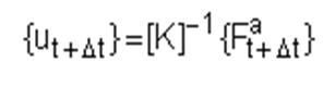
Inertia effects of mass and damping ([C] and [M]) are typically not included for implicit time integration. Average acceleration – displacements evaluated at time t+Δt are given by:

For linear problems, the solution is unconditionally stable when the stiffness matrix [K] is linear, and large time steps can be taken.
For nonlinear problems:
· The solution is obtained using a series of linear approximations (Newton-Raphson method).
· The solution requires inversion of the nonlinear stiffness matrix [K].
· Small iterative time steps are required to achieve convergence.
· Convergence tools are provided, but convergence is not guaranteed for highly nonlinear problems.
A.1.2. Explicit Time Integration
For the explicit method, a central difference time integration method is used. Accelerations evaluated at time t are given by:

For nonlinear problems:
· A lumped mass matrix is required for simple inversion.
· The equations become uncoupled and can be solved for directly (explicitly).
· No inversion of the stiffness matrix is required. All nonlinearities (including contact) are included in the internal force vector.
· The major computational expense is in calculating the internal forces.
· No convergence checks are needed since the equations are uncoupled.
· Very small time steps are required to maintain the stability limit.
A.2. Stability Limit
www.kxcad.net Home > CAE Index > ANSYS Index > Release 11.0 Documentation for ANSYS
A.2.1. Implicit Method
For linear problems, the implicit solution is always stable; that is, the time step can be arbitrarily large.
For nonlinear problems, the time step size may become small due to convergence difficulties.
A.2.2. Explicit Method
The explicit solution is only stable if the time step size is smaller than the critical time step size:

where ωmax = largest natural circular frequency.
Due to this very small time step size, the explicit method is useful only for very short transients.
A.3. Critical Time Step Size of a Rod
www.kxcad.net Home > CAE Index > ANSYS Index > Release 11.0 Documentation for ANSYS
The critical time step is based on the Courant-Friedrichs-Levy criterion. As an example, we will compute the critical time step size of a rod.
The natural frequency is given by:

Δt is the time needed for the wave to propagate through the rod of length l. Note that the critical time step size for explicit time integration depends on element length and material properties (sonic speed).
A.4. ANSYS LS-DYNA Time Step Size
www.kxcad.net Home > CAE Index > ANSYS Index > Release 11.0 Documentation for ANSYS
ANSYS LS-DYNA checks all elements when calculating the required time step. For stability reasons, a scale factor of 0.9 (default) is used to decrease the time step:


